Page 12 - AEI Insights 2018 Vol 4 Issue 1

Furuoka et al, 2018

million in 2017. By contrast, its exports to the EU dropped from US$7,464 million in 2010 to
US$7,397 million in 2015, and only slightly rebounded back to US$7,654 million in 2017
(International Monetary Fund, 2017).

The shifting trends in Singapore’s exports to China and the EU, as elaborated above, have
raised the question of whether the country’s current export practices have a positive effect on
its economic development. In this study, focus is given on the relationship between the amount
of exports and Gross Domestic Product (GDP). Details of the data collection and data analysis
procedures adopted in the study are described in the following section.

Data and Methods

This paper has selected Singapore as a case study to examine the country’s exports to China
and EU and its contribution to economic growth in Singapore for the period of 1975Q1-
2017Q3. Statistics on Singapore’s exports to China and the EU were obtained from the database
on the Direction of Trade (International Monetary Fund, 2017). On the other hand, GDP figures
were sourced from Statistics Singapore (2017). All data on exports and income were
transformed into natural logarithms.

For the purpose of empirical analysis, three econometric methods were employed, namely the
Phillips-Perron (PP) unit root test, the Johansen cointegration test and the Granger causality
test. In the first stage of empirical analysis, the Phillips-Perron unit root test was based on the
following equation (Phillips and Perron, 1988):

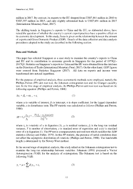
 y     y t1   (1)
0
t
t

where yt is variable of interest, β0 is intercept, α is slope coefficient for the lagged dependent
variable, εt is disturbance term. The PP statistic was calculated as follows (Phillips and Perron,
1988):

 T f (   )( se( ))
pp  t ( 0 ) 2 / 1  0 0 (2)

f 0 f 2 0 2 / 1 s

where tα is t-statistic of α in Equation (1), γ0 is residual variance, f0 is the long-run residual
variance, T is number of observation, s is standard error of regression and se(α) is standard
error of α in Equation (1). The PP test is a nonparametric unit root test which modifies the ADF
statistics (Dickey and Fuller, 1979). In this PP statistic, the presence of serial correlation does
not affect the asymptotic distribution of t-statistic (Phillips and Perron, 1988). The bandwidth
length is determined by the Newey-West method.

In the second stage of empirical analysis, this study relied on the Johansen cointegration test to
examine the long-run relationship between variables. Johansen (1991) proposed a Vector
Autoregression (VAR) for the analysis of cointegration. The Johansen test is based on the
following VAR:

p
y      i y t i   (3)
t
t
i1

12