Page 10 - AEI Insights 2019 - Vol. 5, Issue 1
P. 10
AEI Insights, Vol 5, Issue 1, 2019
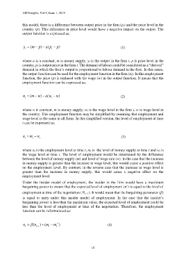
this model, there is a difference between output price in the firm (pi) and the price level in the
country (p). This difference in price level would have a negative impact on the output. The
output function is expressed as;
y (m p (p ) p (1)
) a
i
i
where a is a constant, m is money supply, yi is the output in the firm i, p is price level in the
country, pi is output price in the firm i. The demand of labour could be considered as a “derived”
demand in which the firm’s output is proportional to labour demand in the firm. In this sense,
the output function can be used for the employment function in the firm (ni). In this employment
function, the price (p) is replaced with the wage (w) in the output function. It means that the
employment function can be expressed as;
n (m w ) a (w ) w (2)
i
i
where α is constant, m is money supply, wi is the wage level in the firm i, w is wage level in
the country. This employment function may be simplified by assuming that employment and
wage level is the same in all firms. In this simplified version, the level of employment at time
t can be expressed as;
n m w (3)
t
t
t
where nt is the employment level at time t, mt is the level of money supply at time t and wt is
the wage level at time t. The level of employment would be determined by the difference
between the level of money supply (m) and level of wage rate (w). In the case that the increase
in money supply is greater than the increase in wage level, this would cause a positive effect
on the employment level. By contrast, in the reverse case that the increase in wage level is
greater than the increase in money supply, this would cause a negative effect on the
employment level.
Under the insider model of employment, the insider in the firm would have a maximum
e
bargaining power to ensure that the expected level of employment (n ) is equal to the level of
employment at time of the negotiation ( n 1 t ). It would mean that the bargaining parameter (β)
is equal to unity under this insider model of employment. In the case that the insider’s
bargaining power is less than the maximum value, the expected level of employment could be
less than the level of employment at time of the negotiation. Therefore, the employment
function can be reformulated as:
n (n t 1 ) (m m t e ) (4)
t
t
10

